MuSiC: Multi-subject Single-cell Deconvolution
Xuran Wang
SEAVER Autism Center, Icahn Medical School of Mount Sinai, New York, USASource:
vignettes/MuSiC.Rmd
MuSiC.Rmd
Introduction
This vignette provides a walk through tutorial on how to use
MuSiC to estimate cell type proportions from bulk
sequencing data based on multi-subject single cell data by reproducing
the analysis in MuSiC paper, now is published on Nature
Communications.
Installation
To run the entire deconvolution tutorial, users need to install the
MuSiC
package.
# install devtools if necessary
install.packages('devtools')

# install the MuSiC package
devtools::install_github('xuranw/MuSiC')

# load
library(MuSiC)
Data
MuSiC uses two types of input data:
Bulk expression obtained from RNA sequencing, which is a mixture expression of various cell types. These are the data we want to deconvolve.
Multi-subject single cell expression obtained from single-cell RNA sequencing (scRNA-seq). The cell types of scRNA-seq are pre-determined. These serve as reference for estimating cell type proportions of bulk data.
MuSiC requires raw read counts for both bulk and
single-cell expression. The discussion of the usage of RPKM and TPM can
be found in the Discussion section of our paper.
MuSiC Deconvolution
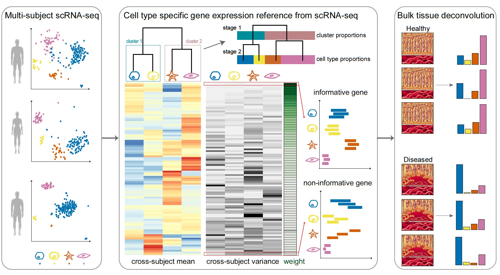
MuSiC utilizes cell-type specific gene expression from single-cell RNA sequencing (RNA-seq) data to characterize cell type compositions from bulk RNA-seq data in complex tissues. By appropriate weighting of genes showing cross-subject and cross-cell consistency, MuSiC enables the transfer of cell type-specific gene expression information from one dataset to another.
Solid tissues often contain closely related cell types which leads to collinearity. To deal with collinearity, MuSiC employs a tree-guided procedure that recursively zooms in on closely related cell types. Briefly, we first group similar cell types into the same cluster and estimate cluster proportions, then recursively repeat this procedure within each cluster.
Sample Analysis
Data Summary
This vignette reproduces the human pancreatic islet and the mouse kidney analysis, which require single cell and bulk RNA-seq datasets from following sources:
| Datasets | Segerstolpe et al. (2016) | Xin et al. (2016) | Fadista et al. (2014) | Park et al. (2018) | Beckerman et al. (2017) |
|---|---|---|---|---|---|
| Session Num. | E-MTAB-5061 | GSE81608 | GSE50244 | GSE107585 | GSE81492 |
| Data type | scRNA-seq | scRNA-seq | bulk RNA-seq | scRNA-seq | bulk RNA-seq |
| Protocol | Smart-seq2 | Illumina HiSeq 2500 | Illumina HiSeq 2000 | 10x | Illumina HiSeq 2500 |
| Tissue | human pancreas | human pancreas | human pancreas | mouse kidney | mouse kidney |
| # of genes | 25,453 | 39,849 | 56,638 | 16,273 | 19,033 |
| # of cells | 2,209 | 1,492 | NA | 43,745 | NA |
| # of cell types | 14 + 1 NA | 4 | NA | 14 + 2 novel | NA |
| # of subjects | 10 (6 healthy + 4 T2D) | 18 (12 healthy + 6 T2D) | 89 | 7 | 10 (6 control + 4 APOL1) |
Bioconductor base package provides
ExpressionSet class, which is a convenient data structure
to hold expression data along with sample/feature annotation. Here we
use two ExpressionSet objects to handle the bulk and single
cell data respectively. The details of constructing
ExpressionSet can be found on this
page. Please see the answer of this Issue for a simple
guidance.
Datasets described in the table above are
all in the form of ExpressionSet and available at the data download page.
UPDATE: Per users’ requests, we have updated
MuSiCfunctions (version 1.0.0) andSingleCellExperimentobjects are used to handle single cell references, where sparse matrices are compatible as read counts. The details of constructingSingleCellExperimentobjects can be found on this page.Datasets described in the table above are in
SingleCellExperiment(single cell references) orExpressionSet(bulk). They are available at the data download page.
Estimation of cell type proportions
Instead of selecting marker genes, MuSiC gives weights to each gene. The weighting scheme is based on cross-subject variation: up-weigh genes with low variation and down-weigh genes with high variation. Here we demonstrate step by step with the human pancreas datasets.
Data Preparations
Bulk data of human pancreas
The dataset from Fadista et al. (2014) contains raw read counts data from bulk RNA-seq of human pancreatic islets to study glucose metabolism in healthy and hyper-hypoglycemic conditions. For the purpose of this vignette, the dataset is pre-processed and made available on the data download page. In addition to read counts, this dataset also contains HbA1c levels, BMI, gender and age information for each subject.
GSE50244.bulk.eset = readRDS('https://xuranw.github.io/MuSiC/data/GSE50244bulkeset.rds')
GSE50244.bulk.eset
#ExpressionSet (storageMode: lockedEnvironment)
#assayData: 32581 features, 89 samples
#  element names: exprs
#protocolData: none
#phenoData
#  sampleNames: Sub1 Sub2 ... Sub89 (89 total)
#  varLabels: sampleID SubjectName ... tissue (7 total)
#  varMetadata: labelDescription
#featureData: none
#experimentData: use 'experimentData(object)'
#Annotation:
bulk.mtx = exprs(GSE50244.bulk.eset)
bulk.meta = exprs(GSE50244.bulk.eset)
Single cell data of human pancreas
The single cell data are from Segerstolpe et
al. (2016), which constrains read counts for 25453 genes across
2209 cells. Here we only include the 1097 cells from 6 healthy subjects.
The read counts are available on the data
download page, in the form of an
SingleCellExperiment.
# Download EMTAB single cell dataset from Github
EMTAB.sce = readRDS('https://xuranw.github.io/MuSiC/data/EMTABsce_healthy.rds')
EMTAB.sce
#class: SingleCellExperiment
#dim: 25453 1097
#metadata(0):
#assays(1): counts
#rownames(25453): SGIP1 AZIN2 ... KIR2DL2 KIR2DS3
#rowData names(1): gene.name
#colnames(1097): AZ_A10 AZ_A11 ... HP1509101_P8 HP1509101_P9
#colData names(4): sampleID SubjectName cellTypeID cellType
#reducedDimNames(0):
#mainExpName: NULL
#altExpNames(0):
Another single cell data is from Xin et al.
(2016), which have 39849 genes and 1492 cells. The read counts
are available on the data download page,
in the form of an ExpressionSet.
# Download Xin et al. single cell dataset from Github
XinT2D.sce = readRDS('https://xuranw.github.io/MuSiC/data/XinT2Dsce.rds')
XinT2D.sce
#class: SingleCellExperiment
#dim: 39849 1492
#metadata(0):
#assays(1): counts
#rownames(39849): A1BG A2M ... LOC102724004 LOC102724238
#rowData names(1): gene.name
#colnames(1492): Sample_1 Sample_2 ... Sample_1491 Sample_1492
#colData names(5): sampleID SubjectName cellTypeID cellType Disease
#reducedDimNames(0):
#mainExpName: NULL
#altExpNames(0):
Bulk Tissue Cell Type Estimation
The deconvolution of 89 subjects from Fadista
et al. (2014) are preformed with bulk data
GSE50244.bulk.eset and single cell reference
EMTAB.eset. We constrained our estimation on 6 major cell
types: alpha, beta, delta, gamma, acinar and ductal, which make up over
90% of the whole islet.
The cell type proportions are estimated by the function music_prop. The
essential inputs are
-
bulk.eset: ExpressionSet of bulk data; -
sc.eset: ExpressionSet of annotated single cell data; -
markers: vector or list of gene names, default asNULL. IfNULL, then use all genes that overlapping in bulk and single-cell dataset; -
clusters: character, must be one of the column names of the phenoData from single cell data, used as clusters; -
samples: character, must be one of the column names of the phenoData from single cell data, used as samples; -
select.ctvector of cell types included for deconvolution, default asNULL. IfNULL, then use all cell types that provided by single-cell dataset. -
verboselogical that toggles log messages.
The function music_prop provides
output as a list with elements:
-
Est.prop.weighted: data.frame of MuSiC estimated proportions, subjects by cell types; -
Est.prop.allgene: data.frame of NNLS estimated proportions, subjects by cell types; -
Weight.gene: matrix, MuSiC estimated weight for each gene, genes by subjects; -
r.squared.full: vector of R squared from MuSiC estimated proportions for each subject; -
Var.prop: matrix of variance of MuSiC estimates.
The estimated proportions are normalized to sum to 1 across included
cell types. Here we use GSE50244.bulk.eset as the
bulk.eset input and EMTAB.eset as
sc.eset input. The clusters is specified as
cellType while samples is
sampleID. As stated before, we only included 6 major cell
types as select.ct.
# Bulk expression matrix
bulk.mtx = exprs(GSE50244.bulk.eset)

# Estimate cell type proportions
Est.prop.GSE50244 = music_prop(bulk.mtx = bulk.mtx, sc.eset = EMTAB.sce, clusters = 'cellType',
                               samples = 'sampleID', select.ct = c('alpha', 'beta', 'delta', 'gamma',
                                                                   'acinar', 'ductal'), verbose = F)
names(Est.prop.GSE50244)
#[1] "Est.prop.weighted" "Est.prop.allgene"  "Weight.gene"       "r.squared.full"    "Var.prop"
Here we use Jitter_Est to
show the difference between different estimation methods.
# Jitter plot of estimated cell type proportions
jitter.fig = Jitter_Est(list(data.matrix(Est.prop.GSE50244$Est.prop.weighted),
                             data.matrix(Est.prop.GSE50244$Est.prop.allgene)),
                        method.name = c('MuSiC', 'NNLS'), title = 'Jitter plot of Est Proportions')

# A more sophisticated jitter plot is provided as below. We seperated the T2D subjects and normal
#subjects by their HbA1c levels.

m.prop.GSE50244 = rbind(melt(Est.prop.GSE50244$Est.prop.weighted),
                        melt(Est.prop.GSE50244$Est.prop.allgene))

colnames(m.prop.GSE50244) = c('Sub', 'CellType', 'Prop')
m.prop.GSE50244$CellType = factor(m.prop.GSE50244$CellType, levels = c('alpha', 'beta', 'delta', 'gamma', 'acinar', 'ductal'))
m.prop.GSE50244$Method = factor(rep(c('MuSiC', 'NNLS'), each = 89*6), levels = c('MuSiC', 'NNLS'))
m.prop.GSE50244$HbA1c = rep(GSE50244.bulk.eset$hba1c, 2*6)
m.prop.GSE50244 = m.prop.GSE50244[!is.na(m.prop.GSE50244$HbA1c), ]
m.prop.GSE50244$Disease = factor(c('Normal', 'T2D')[(m.prop.GSE50244$HbA1c > 6.5)+1], levels = c('Normal', 'T2D'))
m.prop.GSE50244$D = (m.prop.GSE50244$Disease == 'T2D')/5
m.prop.GSE50244 = rbind(subset(m.prop.GSE50244, Disease == 'Normal'), subset(m.prop.GSE50244, Disease != 'Normal'))

jitter.new = ggplot(m.prop.GSE50244, aes(Method, Prop)) +
  geom_point(aes(fill = Method, color = Disease, stroke = D, shape = Disease),
             size = 2, alpha = 0.7, position = position_jitter(width=0.25, height=0)) +
  facet_wrap(~ CellType, scales = 'free') + scale_colour_manual( values = c('white', "gray20")) +
  scale_shape_manual(values = c(21, 24))+ theme_minimal()

plot_grid(jitter.fig, jitter.new, labels = 'auto')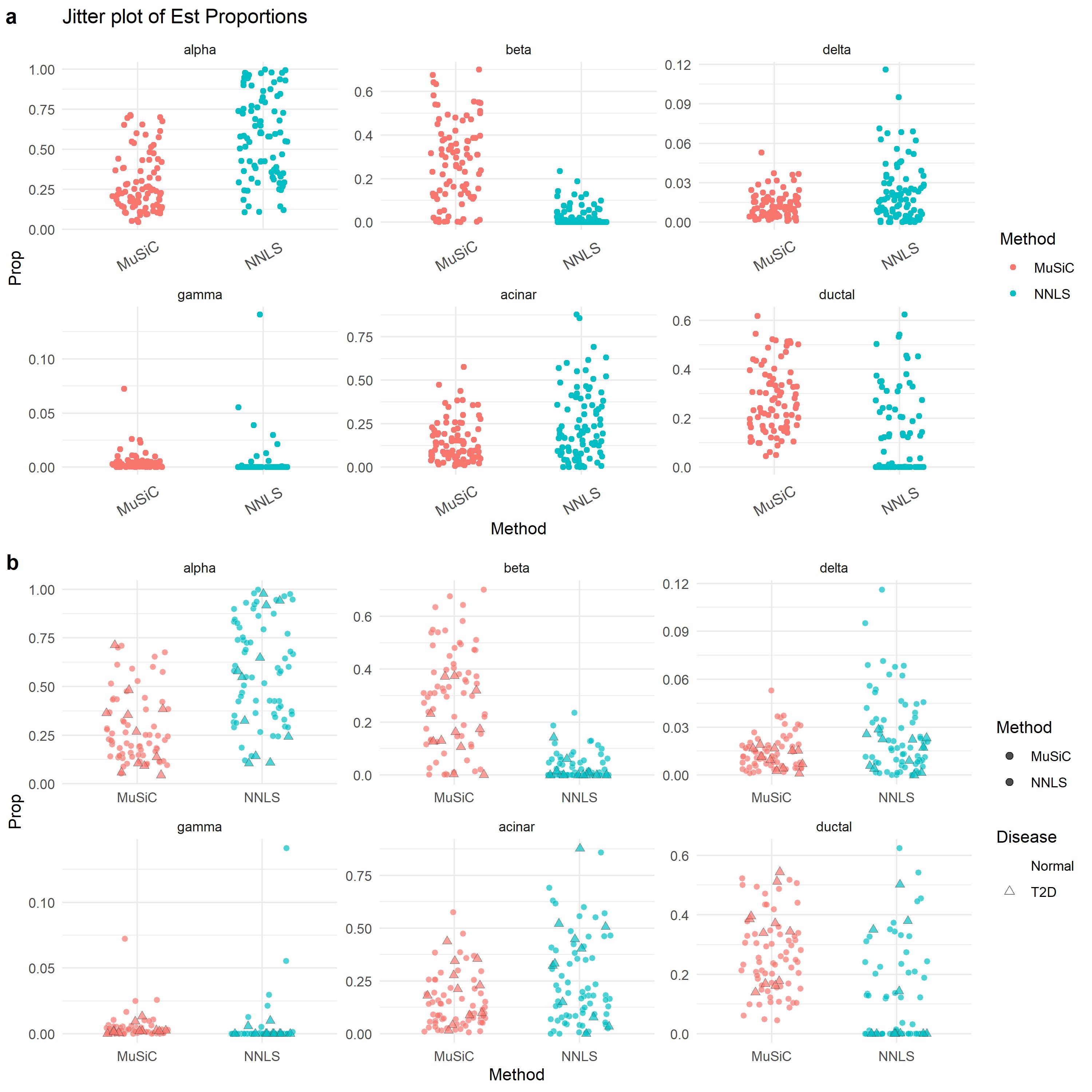
It is well known that the beta cell proportions is related to T2D disease status. In the progress of T2D, the number of beta cells decreases. One of the most important test for T2D is HbA1c (hemoglobin A1c) test. When HbA1c level is greater than 6.5%, the patient is diagnosed as T2D. Let’s look at the beta cell proportions with HbA1c level.
# Create dataframe for beta cell proportions and HbA1c levels
m.prop.ana = data.frame(pData(GSE50244.bulk.eset)[rep(1:89, 2), c('age', 'bmi', 'hba1c', 'gender')],
                        ct.prop = c(Est.prop.GSE50244$Est.prop.weighted[, 2],
                                    Est.prop.GSE50244$Est.prop.allgene[, 2]),
                        Method = factor(rep(c('MuSiC', 'NNLS'), each = 89),
                        levels = c('MuSiC', 'NNLS')))
colnames(m.prop.ana)[1:4] = c('Age', 'BMI', 'HbA1c', 'Gender')
m.prop.ana = subset(m.prop.ana, !is.na(HbA1c))
m.prop.ana$Disease = factor( c('Normal', 'T2D')[(m.prop.ana$HbA1c > 6.5) + 1], c('Normal', 'T2D') )
m.prop.ana$D = (m.prop.ana$Disease == 'T2D')/5

ggplot(m.prop.ana, aes(HbA1c, ct.prop)) +
  geom_smooth(method = 'lm',  se = FALSE, col = 'black', lwd = 0.25) +
  geom_point(aes(fill = Method, color = Disease, stroke = D, shape = Disease), size = 2, alpha = 0.7) +  facet_wrap(~ Method) +
  ggtitle('HbA1c vs Beta Cell Type Proportion') + theme_minimal() +
  scale_colour_manual( values = c('white', "gray20")) +
  scale_shape_manual(values = c(21, 24))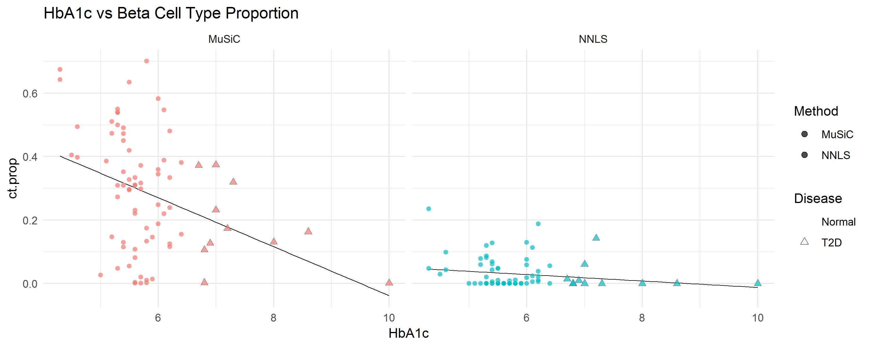
The numerical evaluation can be obtained by linear regression. There is a significant negative correlation between HbA1c levels and beta cell proportions, after adjusted Age, BMI and Gender.
lm.beta.MuSiC = lm(ct.prop ~ HbA1c + Age + BMI + Gender, data = subset(m.prop.ana, Method == 'MuSiC'))
lm.beta.NNLS = lm(ct.prop ~ HbA1c + Age + BMI + Gender, data = subset(m.prop.ana, Method == 'NNLS'))
summary(lm.beta.MuSiC)
#
#Call:
#lm(formula = ct.prop ~ HbA1c + Age + BMI + Gender, data = subset(m.prop.ana,
#    Method == "MuSiC"))
#
#Residuals:
#     Min       1Q   Median       3Q      Max
#-0.27768 -0.13186 -0.01096  0.10661  0.35790
#
#Coefficients:
#              Estimate Std. Error t value Pr(>|t|)
#(Intercept)   0.877022   0.190276   4.609 1.71e-05 ***
#HbA1c        -0.061396   0.025403  -2.417   0.0182 *
#Age           0.002639   0.001772   1.489   0.1409
#BMI          -0.013620   0.007276  -1.872   0.0653 .
#GenderFemale -0.079874   0.039274  -2.034   0.0457 *
#---
#Signif. codes:  0 '***' 0.001 '**' 0.01 '*' 0.05 '.' 0.1 ' ' 1
#
#Residual standard error: 0.167 on 72 degrees of freedom
#Multiple R-squared:  0.2439,   Adjusted R-squared:  0.2019
#F-statistic: 5.806 on 4 and 72 DF,  p-value: 0.0004166

summary(lm.beta.NNLS)
#
#Call:
#lm(formula = ct.prop ~ HbA1c + Age + BMI + Gender, data = subset(m.prop.ana,
#    Method == "NNLS"))
#
#Residuals:
#     Min       1Q   Median       3Q      Max
#-0.04671 -0.02918 -0.01795  0.01394  0.19362
#
#Coefficients:
#               Estimate Std. Error t value Pr(>|t|)
#(Intercept)   0.0950960  0.0546717   1.739   0.0862 .
#HbA1c        -0.0093214  0.0072991  -1.277   0.2057
#Age           0.0005268  0.0005093   1.035   0.3044
#BMI          -0.0015116  0.0020906  -0.723   0.4720
#GenderFemale -0.0037650  0.0112844  -0.334   0.7396
#---
#Signif. codes:  0 '***' 0.001 '**' 0.01 '*' 0.05 '.' 0.1 ' ' 1
#
#Residual standard error: 0.04799 on 72 degrees of freedom
#Multiple R-squared:  0.0574,   Adjusted R-squared:  0.005028
#F-statistic: 1.096 on 4 and 72 DF,  p-value: 0.3651
Estimation of cell type proportions with pre-grouping of cell types
Solid tissues often contain closely related cell types, and correlation of gene expression between these cell types leads to collinearity, making it difficult to resolve their relative proportions in bulk data. To deal with collinearity, MuSiC employs a tree-guided procedure that recursively zooms in on closely related cell types. Briefly, we first group similar cell types into the same cluster and estimate cluster proportions, then recursively repeat this procedure within each cluster. At each recursion stage, we only use genes that have low within-cluster variance, a.k.a. the cross-cell consistent genes. This is critical as the mean expression estimates of genes with high variance are affected by the pervasive bias in cell capture of scRNA-seq experiments, and thus cannot serve as reliable reference.
We demonstrate this procedure by reproducing the analysis of mouse kidney in MuSiC paper.
Data Preparation
Bulk data
The dataset GEO
entry (GSE81492) (see Beckerman et al.
2017) contains raw RNA-seq and sample annotation data. For the
purpose of this vignette, we will use the read counts data
Mousebulkeset.rds from the data
download page.
# Download Mouse bulk dataset from Github
Mouse.bulk.eset = readRDS('https://xuranw.github.io/MuSiC/data/Mousebulkeset.rds')
Mouse.bulk.eset

#ExpressionSet (storageMode: lockedEnvironment)
#assayData: 19033 features, 10 samples
#  element names: exprs
#protocolData: none
#phenoData
#  sampleNames: control.NA.27 control.NA.30 ... APOL1.GNA78M (10 total)
#  varLabels: sampleID SubjectName Control
#  varMetadata: labelDescription
#featureData: none
#experimentData: use 'experimentData(object)'
#Annotation:
Single cell data
The single cell data are from GEO
entry (GSE107585) (see Park et al.
2018), which constrains read counts for 16273 genes across 43745
cells. Due to the space limitation of Github, only a subset of the read
counts Mousesubeset.rds are available on the data download page, in the form of an
ExpressionSet. This subset contains 16273 genes across
10000 cells.
# Download Mouse single cell dataset from Github
Mousesub.sce = readRDS('https://xuranw.github.io/MuSiC/data/Mousesub_sce.rds')
Mousesub.sce

#class: SingleCellExperiment
#dim: 16273 10000
#metadata(0):
#assays(1): counts
#rownames(16273): Rp1 Sox17 ... DHRSX CAAA01147332.1
#rowData names(0):
#colnames(10000): TGGTTCCGTCGGCTCA-2 CGAGCCAAGCGTCAAG-4 ... GTATTCTGTAGCTAAA-2 GAGCAGAGTCAACATC-1
#colData names(4): sampleID SubjectName cellTypeID cellType
#reducedDimNames(0):
#mainExpName: NULL
#altExpNames(0):

levels(Mousesub.sce$cellType)
# [1] "Endo"     "Podo"     "PT"       "LOH"      "DCT"      "CD-PC"    "CD-IC"    "CD-Trans" "Novel1"
#[10] "Fib"      "Macro"    "Neutro"   "B lymph"  "T lymph"  "NK"       "Novel2"
Notice that the single cell dataset has 16 cell types, including 2 novel cell types and a transition cell type (CD-Trans). We exclude those 3 cell types in our analysis.
Estimation of cell type proportions
Clustering single cell data
In previous MuSiC
estimation procedure, the first step is to produce design matrix,
cross-subject mean of relative abundance, cross-subject variance of
relative abundance and average library size from single cell reference.
These are taken care of by the function music_basis. The
essential inputs of music_basis
are:
-
x: ExpressionSet of single cell dataset; -
non.zero: logical, default asTRUE. If true, remove all genes with zero expression; -
markers: vector or list of gene names. Default asNULL. IfNULL, then use all genes provided byx; -
clusters: character, must be one of the column names of the phenoData from single cell data, used as clusters; -
samples: character, must be one of the column names of the phenoData from single cell data, used as samples; -
select.ctvector of cell types included for deconvolution, default asNULL. IfNULL, then use all cell types that provided by single-cell dataset. -
verboselogical that toggles log messages.
The outputs of music_basis is a
list of elements:
-
Disgn.mtx: gene by cell type matrix of design matrix; -
S: subject by cell type matrix of library size; -
M.S: vector of average library size for each cell type; -
M.theta: gene by cell type matrix of average relative abundance; -
Sigma: gene by cell type matrix of cross-subject variation.
We next use the hclust function to get a tree0based
clustering of the cell types using the cross-subject mean matrix and the
design matrix.
# Produce the first step information
Mousesub.basis = music_basis(Mousesub.sce, clusters = 'cellType', samples = 'sampleID',
                             select.ct = c('Endo', 'Podo', 'PT', 'LOH', 'DCT', 'CD-PC', 'CD-IC', 'Fib',
                                           'Macro', 'Neutro','B lymph', 'T lymph', 'NK'))

# Plot the dendrogram of design matrix and cross-subject mean of realtive abundance
par(mfrow = c(1, 2))
d <- dist(t(log(Mousesub.basis$Disgn.mtx + 1e-6)), method = "euclidean")
# Hierarchical clustering using Complete Linkage
hc1 <- hclust(d, method = "complete" )
# Plot the obtained dendrogram
plot(hc1, cex = 0.6, hang = -1, main = 'Cluster log(Design Matrix)')
d <- dist(t(log(Mousesub.basis$M.theta + 1e-8)), method = "euclidean")
# Hierarchical clustering using Complete Linkage
# hc2 <- hclust(d, method = "complete" )
hc2 <- hclust(d, method = "complete")
# Plot the obtained dendrogram
plot(hc2, cex = 0.6, hang = -1, main = 'Cluster log(Mean of RA)')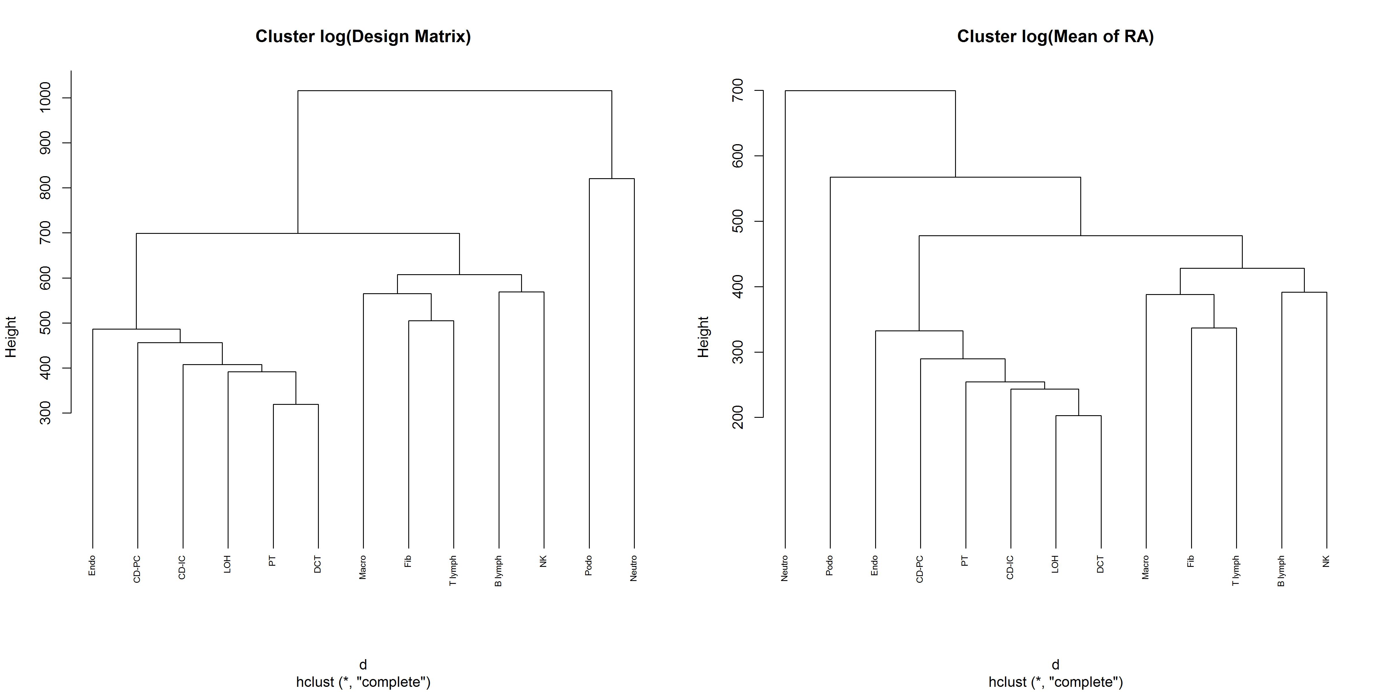
The immune cells are clustered together and the kidney specific cells are clustered together. Notice that DCT and PT are within the same high-level grouping. The cut-off is user determined. Here we cut 13 cell types into 4 groups:
- Group 1: Neutro
- Group 2: Podo
- Group 3: Endo, CD-PC, CD-IC, LOH, DCT, PT
- Group 4: Fib, Macro, NK, B lymph, T lymph
The tree-guided recursive estimation for mouse kidney analysis includes 2 steps:
- Step 1. Estimate proportions of each high level cluster; \((p_1,p_2,p_3,p_4)\)
- Step 2. Estimate cell type proportions within each cluster; \((p_{31},p_{32},.,p_{36},p_{41},.,p_{45})\)
Bulk Tissue Cell Type Estimation with Pre-grouping of Cell Types
We manually specify the cluster and annotated single cell data with cluster information.
clusters.type = list(C1 = 'Neutro', C2 = 'Podo', C3 = c('Endo', 'CD-PC', 'LOH', 'CD-IC', 'DCT', 'PT'), C4 = c('Macro', 'Fib', 'B lymph', 'NK', 'T lymph'))

cl.type = as.character(Mousesub.sce$cellType)

for(cl in 1:length(clusters.type)){
  cl.type[cl.type %in% clusters.type[[cl]]] = names(clusters.type)[cl]
}
Mousesub.sce$clusterType = factor(cl.type, levels = c(names(clusters.type), 'CD-Trans', 'Novel1', 'Novel2'))

# 13 selected cell types
s.mouse = unlist(clusters.type)
s.mouse
#       C1        C2       C31       C32       C33       C34       C35       C36       C41       C42
# "Neutro"    "Podo"    "Endo"   "CD-PC"     "LOH"   "CD-IC"     "DCT"      "PT"   "Macro"     "Fib"
#      C43       C44       C45
#"B lymph"      "NK" "T lymph"
We then select genes that are differentially expressed within cluster
C3 (Epithelial cells) and C4 (Immune cells),
available on data download page. Function
music_prop.cluster
is used for estimation with pre-clustering of cell types. The essential
inputs are the same as music_prop except two unique inputs:
groups and group.markers. groups
passes the column name of higher-cluster in phenoData. The intra-cluster
differentially expressed genes are passed by
group.marker.
load('https://xuranw.github.io/MuSiC/data/IEmarkers.RData')
# This RData file provides two vectors of gene names Epith.marker and Immune.marker

# We now construct the list of group marker
IEmarkers = list(NULL, NULL, Epith.marker, Immune.marker)
names(IEmarkers) = c('C1', 'C2', 'C3', 'C4')
# The name of group markers should be the same as the cluster names

Est.mouse.bulk = music_prop.cluster(bulk.mtx = exprs(Mouse.bulk.eset), sc.sce = Mousesub.sce, group.markers = IEmarkers, clusters = 'cellType', groups = 'clusterType', samples = 'sampleID', clusters.type = clusters.type)
Due to the limited space of Github, we can only demo
music_prop.cluster with a subset of mouse kidney single
cell dataset. Therefore, the results might be different from the one
presented in the paper due to incomplete reference single cell
dataset.
Benchmark Evaluation
Benchmark dataset is constructed by summing up single cell data from
XinT2D.eset. The artificial bulk data is constructed
through function bulk_construct.
The inputs are single cell dataset, cluster name
(clusters), sample name (samples) and selected
cell type (select.ct). bulk_construct
returns a ExpressionSet of artificial bulk dataset
Bulk.counts and a matrix of real cell type counts
num.real.
# Construct artificial bulk dataset. Use all 4 cell types: alpha, beta, gamma, delta
XinT2D.construct.full = bulk_construct(XinT2D.sce, clusters = 'cellType', samples = 'SubjectName')

names(XinT2D.construct.full)
# [1] "bulk.counts" "num.real"

dim(XinT2D.construct.full$bulk.counts)
#[1] 39849    18
# 39849 genes * 18 samples
XinT2D.construct.full$bulk.counts[1:5, 1:5]
#      Non T2D 1 Non T2D 2 Non T2D 3 Non T2D 5 Non T2D 6
#A1BG        297       269       127      1042       262
#A2M           1         1        19        21         2
#A2MP1       493         0         0         0         0
#NAT1       1856        36       278       559      1231
#NAT2          1         0         0         0         0

head(XinT2D.construct.full$num.real)
#          alpha beta delta gamma
#Non T2D 1    53   13     5     3
#Non T2D 2     4   13     2     5
#Non T2D 3    27   10     3     2
#Non T2D 4    14   10     0     3
#Non T2D 5    23   22     5     2
#Non T2D 6    36    7     4     1

# calculate cell type proportions
XinT2D.construct.full$prop.real = relative.ab(XinT2D.construct.full$num.real, by.col = FALSE)
head(XinT2D.construct.full$prop.real)
#              alpha      beta      delta      gamma
#Non T2D 1 0.7162162 0.1756757 0.06756757 0.04054054
#Non T2D 2 0.1666667 0.5416667 0.08333333 0.20833333
#Non T2D 3 0.6428571 0.2380952 0.07142857 0.04761905
#Non T2D 4 0.5185185 0.3703704 0.00000000 0.11111111
#Non T2D 5 0.4423077 0.4230769 0.09615385 0.03846154
#Non T2D 6 0.7500000 0.1458333 0.08333333 0.02083333
The estimation of cell type proportions:
# Estimate cell type proportions of artificial bulk data
Est.prop.Xin = music_prop(bulk.mtx = XinT2D.construct.full$bulk.counts, sc.sce = EMTAB.sce,
                          clusters = 'cellType', samples = 'sampleID',
                          select.ct = c('alpha', 'beta', 'delta', 'gamma'))
#Creating Relative Abudance Matrix...
#Creating Variance Matrix...
#Creating Library Size Matrix...
#Used 17884 common genes...
#Used 4 cell types in deconvolution...
#Non T2D 1 has common genes 15115 ...
#Non T2D 2 has common genes 12826 ...
#Non T2D 3 has common genes 13553 ...
#Non T2D 4 has common genes 13491 ...
#Non T2D 5 has common genes 14585 ...
#Non T2D 6 has common genes 13984 ...
#Non T2D 7 has common genes 13065 ...
#Non T2D 8 has common genes 13756 ...
#Non T2D 9 has common genes 13813 ...
#Non T2D 10 has common genes 14566 ...
#Non T2D 11 has common genes 14197 ...
#Non T2D 12 has common genes 15507 ...
#T2D 1 has common genes 14936 ...
#T2D 2 has common genes 15084 ...
#T2D 3 has common genes 14175 ...
#T2D 4 has common genes 16163 ...
#T2D 5 has common genes 15866 ...
#T2D 6 has common genes 15673 ...
The numeric evaluation is conducted by Eval_multi, which
compares the real and estimated cell type proportions by
- root-mean-squared deviation (RMSD);
- mean absolute difference (mAD);
- Pearson’s correlation (R).
The visualization of cell type proportions are provided by Prop_comp_multi,
Abs_diff_multi
and Scatter_multi.
# Estimation evaluation

Eval_multi(prop.real = data.matrix(XinT2D.construct.full$prop.real),
           prop.est = list(data.matrix(Est.prop.Xin$Est.prop.weighted),
                           data.matrix(Est.prop.Xin$Est.prop.allgene)),
           method.name = c('MuSiC', 'NNLS'))

#           RMSD     mAD      R
#MuSiC   0.09881 0.06357 0.9378
#NNLS    0.17161 0.11749 0.8159

library(cowplot)
prop.comp.fig = Prop_comp_multi(prop.real = data.matrix(XinT2D.construct.full$prop.real),
                                prop.est = list(data.matrix(Est.prop.Xin$Est.prop.weighted),
                                                data.matrix(Est.prop.Xin$Est.prop.allgene)),
                                method.name = c('MuSiC', 'NNLS'),
                                title = 'Heatmap of Real and Est. Prop' )

abs.diff.fig = Abs_diff_multi(prop.real = data.matrix(XinT2D.construct.full$prop.real),
                              prop.est = list(data.matrix(Est.prop.Xin$Est.prop.weighted),
                                              data.matrix(Est.prop.Xin$Est.prop.allgene)),
                              method.name = c('MuSiC', 'NNLS'),
                              title = 'Abs.Diff between Real and Est. Prop' )

plot_grid(prop.comp.fig, abs.diff.fig, labels = "auto", rel_widths = c(4,3))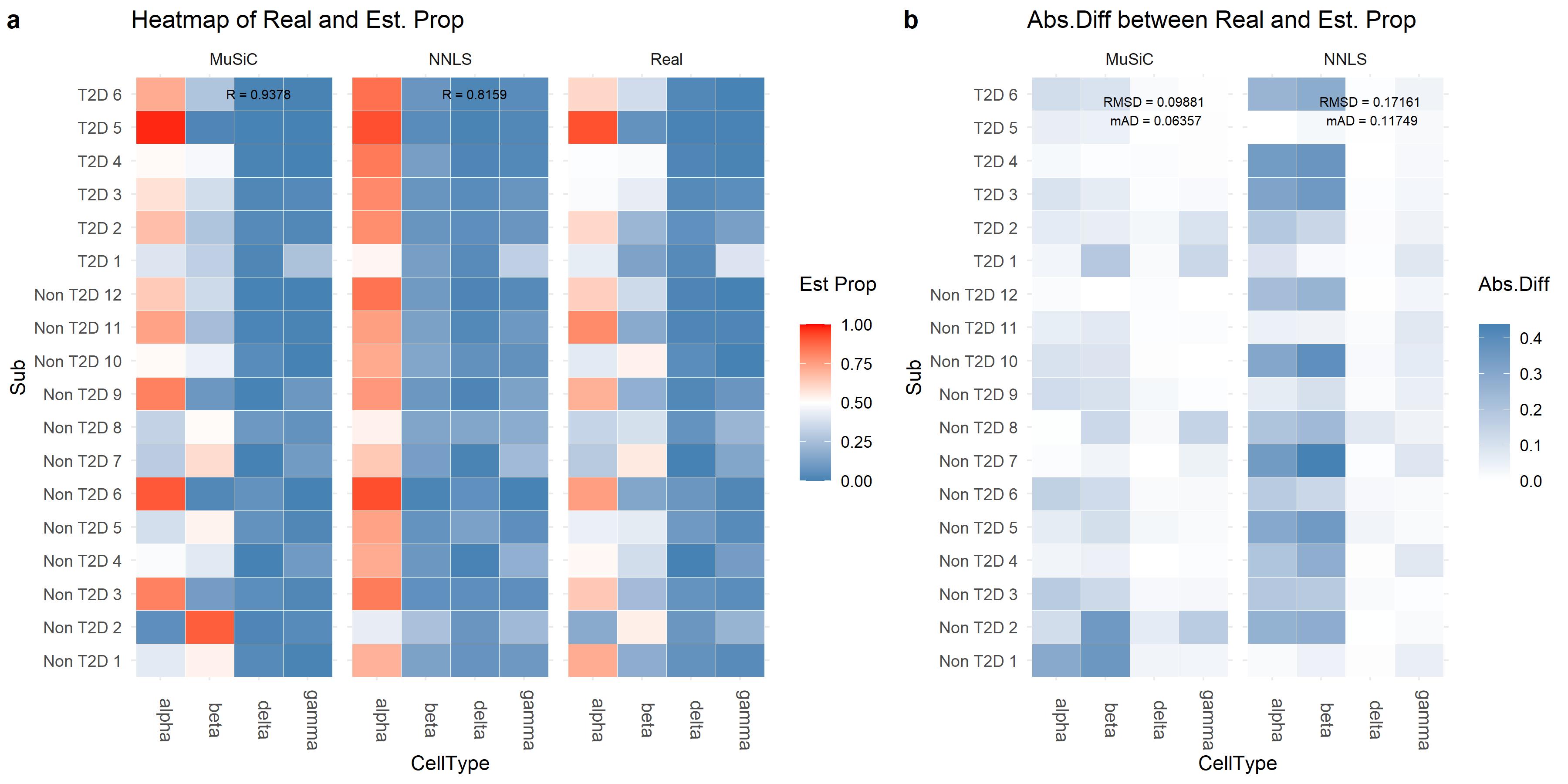
In our paper, we also compared our method with existing methods: CIBERSORT (see Newman et al. 2015) and bseq-sc (see Baron et al. 2016).